Why Go Custom?
Early in the design, I ran into timing problems with the Muller C-elements. These are the foundational cells that make the entire async handshake protocol work, and they contain combinational feedback loops. My initial thought was that it would not be possible to run static timing analysis on a design with these kinds of cells. The feedback loops create circular paths that STA cannot analyze in the traditional sense.
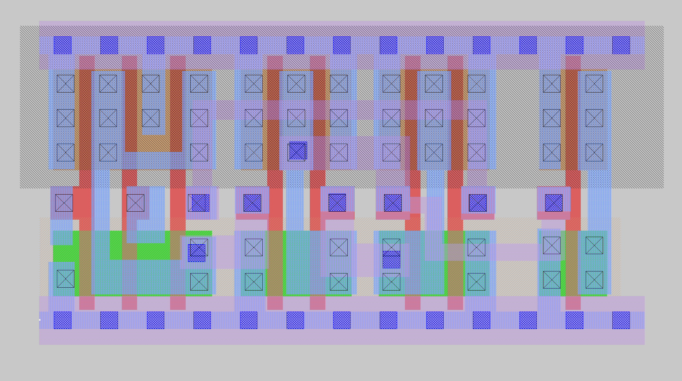
If I could not constrain them in the existing flow, I would need to characterize them myself. That meant building custom cells with Liberty timing models that described their behavior to the timing engine. And that meant going into Magic and drawing layout.
Not Just One C-Element
In the earlier post on synthesis, I talked about C-elements as if there were only one kind. There are actually several variants used throughout the design, each tailored to the needs of a particular piece of control circuitry.
The cell I chose to lay out first was a 3-input asymmetric C-element. "Asymmetric" means the inputs are not equal: the A input overrides the output to 1 if A is low, but to drive the output to 0, all three inputs must agree. Here is the truth table:
| A | B | C | OUT |
|---|---|---|-----|
| 0 | 0 | 0 |  1  |  A low: output high
| 0 | 0 | 1 |  1  |  A low: output high
| 0 | 1 | 0 |  1  |  A low: output high
| 0 | 1 | 1 |  1  |  A low: output high
| 1 | 0 | 0 | OUT |  Hold previous state
| 1 | 0 | 1 | OUT |  Hold previous state
| 1 | 1 | 0 | OUT |  Hold previous state
| 1 | 1 | 1 |  0  |  All high: output low
And the gate-level implementation:
module c_element_bc_n_sc (
    output wire  out,
    input wire   a,
    input wire   b,
    input wire   c
);
    wire out_n;
    wire a_fb_out;
    wire cmb_out;

    primitive_nand3 combiner_gate  (.Y(cmb_out),   .A(a),         .B(b), .C(c));
    primitive_nand2 out_pre_gate   (.Y(out_n),     .A(a_fb_out),  .B(cmb_out));
    primitive_nand2 a_fb_out_gate  (.Y(a_fb_out),  .A(out_n),     .B(a));
    assign out = ~out_n;
endmodule
Magic
Magic is a layout editor that has been around since the 1980s at UC Berkeley. In the open-source flow, it handles custom cell layout, DRC, and parasitic extraction. It is a capable tool that does everything you need.
That said, for someone coming from a tool like Virtuoso, it feels different. The interface has its own way of doing things. Operations that are intuitive in one tool require a different mental model in the other. I will leave the specifics to the reader to discover on their own. It is worth experimenting with. You will develop your own opinion quickly.
My approach was straightforward: grab the existing SKY130 standard cells needed to build a C-element, place them down in Magic, and wire them up, no problem.
The Hard Part
The hard part is making the cell fit onto a standard cell row without every downstream tool complaining.
SKY130 standard cells (like all other standard cells) have strict dimensional requirements. The abutment box and cell origin has to follow a precise grid. The cell boundary must abut all neighboring cells in all orientations without generating DRC errors. Ports have to sit on grid intersections so the router can place vias/contacts cleanly. The substrate diffusion layers (PSDM, NSDM) have to extend to the edges of the abutment box, which sometimes requires GDS post-processing in KLayout after the cell is drawn. Well taps are handled by separate tap cells, so your custom cell exports VPB and VPB ports rather than including internal tap connections.
There are also MOSFET layer substitutions specific to standard cells. You cannot just drop in a regular MOSFET and expect it to work in a standard cell context. The layers are different.
A lot of these learnings are documented in an excellent walkthrough by the Institute for Integrated Circuits at JKU Linz: SKY130 RTL with Custom Standardcell to GDSII. If you are seriously considering drawing your own SKY130 cells, start there. It will save you days of confusion.
Of course I did it the hard way and didn't find this document until afterwards, so I spent an entire week just getting this single cell to fit onto the standard cell row without DRC errors, figuring out how to insert it into the LibreLane flow, and beginning to set up the SPICE simulations. The first one is always the hardest, the follow on cells would go much faster.
Simulation
For schematic capture, the open-source flow provides XSCHEM, which integrates well with the SKY130 PDK and ties directly into ngspice. It is a good tool for this process node.
But since I was working directly with pre-built standard cells, just abutting them and wiring up, it was simpler to use magic to extract the spice netlist from the layout. The circuit is small enough that it is easy to verify correctness by hand.
Running a basic functional simulation in ngspice is straightforward. You write a test bench, apply stimulus, and verify the C-element behaves correctly. That part works fine.
The Wall
The next step after functional verification is characterization. This is where you measure setup time, hold time, and propagation delay across all PVT corners using a table of input slew rates and load capacitances. You build SPICE test benches for each timing arc, run them at every condition and extract the timing numbers. Those numbers go into Liberty timing model tables that the STA engine uses.
This is doable. All the tools are there. ngspice can run the simulations. The SKY130 PDK provides the corner models. The Liberty format is well-documented. Writing up a characterization flow is a one day exercise with current AI tools.
To get a sense of what "characterizing a cell" actually means, here is a snippet from one of the existing SKY130 latches. This is just the timing block for the Q output pin with D as the related input pin:
timing () {
    cell_fall ("del_1_7_7") {
        index_1("0.0100000000, 0.0230506000, 0.0531329000, 0.1224740000, 0.2823110000, 0.6507430000, 1.5000000000");
        index_2("0.0005000000, 0.0013042100, 0.0034019100, 0.0088735700, 0.0231459000, 0.0603741000, 0.1574810000");
        values("0.2059938000, 0.2114576000, 0.2228863000, 0.2459647000, 0.2959996000, 0.4191275000, 0.7398180000", \
            "0.2109205000, 0.2163872000, 0.2278050000, 0.2508747000, 0.3009119000, 0.4239406000, 0.7436882000", \
            "0.2241103000, 0.2295770000, 0.2409953000, 0.2640648000, 0.3141020000, 0.4371303000, 0.7568836000", \
            "0.2554638000, 0.2609310000, 0.2723470000, 0.2954101000, 0.3454567000, 0.4684903000, 0.7887424000", \
            "0.3126409000, 0.3180636000, 0.3295308000, 0.3525625000, 0.4025871000, 0.5256808000, 0.8454011000", \
            "0.4020602000, 0.4074693000, 0.4189192000, 0.4419799000, 0.4920234000, 0.6150448000, 0.9347076000", \
            "0.5430605000, 0.5485234000, 0.5599546000, 0.5830264000, 0.6331188000, 0.7562485000, 1.0771032000");
    }
    cell_rise ("del_1_7_7") { /* 7x7 table of rise delays */ }
    fall_transition ("del_1_7_7") { /* 7x7 table of fall transition times */ }
    rise_transition ("del_1_7_7") { /* 7x7 table of rise transition times */ }
    related_pin : "D";
    timing_sense : "positive_unate";
    timing_type : "combinational";
}
That is one timing arc for one related pin. Each entry in those 7x7 tables comes from a SPICE simulation at a specific input slew rate (index_1) and load capacitance (index_2). For a single cell, you need cell_fall, cell_rise, fall_transition, and rise_transition tables for every related pin combination. That is hundreds of SPICE simulations per cell, per PVT corner. Repeat for every cell in your library.
This is why companies doing this kind of work pay for tools like Synopsys SiliconSmart or Cadence Liberate. These tools automate the entire characterization process: generate the SPICE test benches, dispatch them to a server farm, parse the results, and assemble the Liberty file. The licenses are expensive, the compute is expensive, and the simulations run for days. That is the cost of doing standard cell characterization at production quality.
It was at this point, realizing that I would need to run hundreds of simulations across multiple corners for each cell variant, that the math stopped working. I had one C-element drawn and partially characterized. I needed at least ten different async cell variants: C-elements with different drive strengths, C-elements with reset, mutex cells, arbiter cells. Each one would need its own layout, its own SPICE characterization, and its own Liberty model. Multiply that by the number of PVT corners, and I was looking at weeks of work, and that is if everything "just worked" without a hitch, which it never does.
Tapeout was staring me in the face. This wasn't going to work.
Jumping Ship
So I stopped. I stepped back and dug into whether there was a way to avoid custom cells entirely. That question led directly to the work described in the previous two posts: building C-elements from standard cell gate primitives with hierarchy preservation, and constraining the feedback loops with false paths and per-handshake clock domains.
It turns out STA can handle combinational feedback just fine if you tell it which paths to ignore. The false path approach works. The gate-level C-elements work. They are larger and slower than a hand-drawn custom cell would be, but they are correct, they are constrainable, and they got me to tapeout.
Sometimes doing the wrong thing is what is needed to put you on the path to doing the right thing. I would not have figured out the constraint-based approach without first hitting the wall on custom cells. The week I spent in Magic was not wasted. It taught me exactly how much work custom cells require, and that knowledge informed every decision that followed.
Plugging into LibreLane
One thing worth mentioning: if you do go through the effort of building custom cells, you need to tell LibreLane about them. Magic generates LEF and GDS files for the physical layout. You generate Liberty timing models from your SPICE characterization. And you provide a Verilog behavioral model for simulation. All of these get added to the LibreLane configuration as extra libraries:
# Custom cell files
EXTRA_LEFS:
  - "dir::../analog/custom_cells/lib/async_cells.lef"
EXTRA_GDS_FILES:
  - "dir::../analog/custom_cells/lib/async_cells.gds"
EXTRA_LIBS:
  - "dir::../analog/custom_cells/lib/async_cells__ff_n40C_1v95.lib"
  - "dir::../analog/custom_cells/lib/async_cells__ss_100C_1v60.lib"
  - "dir::../analog/custom_cells/lib/async_cells__tt_025C_1v80.lib"
EXTRA_VERILOG_MODELS:
  - "dir::../analog/custom_cells/lib/async_cells.v"
My plan was to package all of the custom cells into a single library file per view, but these arguments accept a list, so you could add each cell individually if you prefer. One Liberty file per PVT corner (fast-fast, slow-slow, typical), one LEF, one GDS, one Verilog model. That is the interface between your custom cells and the rest of the automated flow.
Respect
If there is one takeaway from this experience, it is this: if you can get away with not drawing custom cells, do it. Use the existing library. Build from gates. Work around the limitations with constraints and hierarchy.
Unless you enjoy this kind of work and have plenty of time to figure it out. Then by all means, go for it. It is a great learning exercise. You will come away with a much deeper understanding of what goes into a standard cell library, and a much greater respect for the cell design and layout teams that build them. That work is nuanced, detail-oriented, and critically important. Every chip ever built rests on the quality of those cells.
But for me, I was trying to get a chip out the door. Whatever gets me there fastest is the path I take. The custom cells will happen on the next chip, when there is time to do them right.